Global Health Policy Simulation model

Quick Start

The Health GPS application provides a Command Line Interface (CLI) and runs on Windows 10 (and newer) and Linux devices. All supported options are provided to the model via a configuration file (JSON format), including population size, intervention scenarios and number of runs. Users are encouraged to start exploring the model by using the included example dataset, changing the provided configuration file, and running the model.

Pre-compiled binaries for Windows and Linux are available on the releases page for generic x86-64 CPUs. If you want a version of the program tailored to your specific CPU (e.g. for HPC) or you wish to develop Health GPS, follow the instructions to build from source in the developer guide. To use the binaries, you will need to unzip the downloaded file to a directory of your choice.

Known Issue: Windows 10 support for VT (Virtual Terminal) / ANSI escape sequences is turned OFF by default, this is required to display colours on console / shell terminals. You can enable this feature manually by editing windows registry keys, however we recommend the use of Windows Terminal, which is a modern terminal application for command-line tools, has no such limitation, and is now distributed as part of the Windows 11 installation.

Example usage

Health GPS requires model configuration files in order to be able to run. These files can either be in a local directory or as a zip file on the local machine or on the web. Here, we will use a model available from the Health-GPS examples repository. (We are assuming that you have changed directories to wherever you have built or extracted the Health-GPS binaries.)

For Windows:

.\HealthGPS.Console.exe -c https://github.com/imperialCHEPI/healthgps-examples/releases/download/20240907/HLM_France.zip

For Linux:

./HealthGPS.Console -c https://github.com/imperialCHEPI/healthgps-examples/releases/download/20240907/HLM_France.zip

Output data will be written to a subfolder of your home directory, healthgps/results/france.

Optional: validate a config without running trials: HealthGPS.Console -c path/to/config.json --dry-run. Limit CPU threads with -T (see performance guide).

Results

NB: For analysis and visualisation of Health GPS output data, we recommend the healthgpsrvis R package, but here we show how to do some analysis manually.

Health-GPS produces output data simultaneously in CSV and JSON (same run; prefer CSV for analysis). Large or FINCH-style configs may also write per-income-stratum CSVs and an optional _IndividualIDTracking.csv. See the User Guide for details.

Analysing the JSON output data

To read JSON files in R, you need the jsonlite package:

require(jsonlite)
data <- fromJSON(result_filename.json)
View(data)

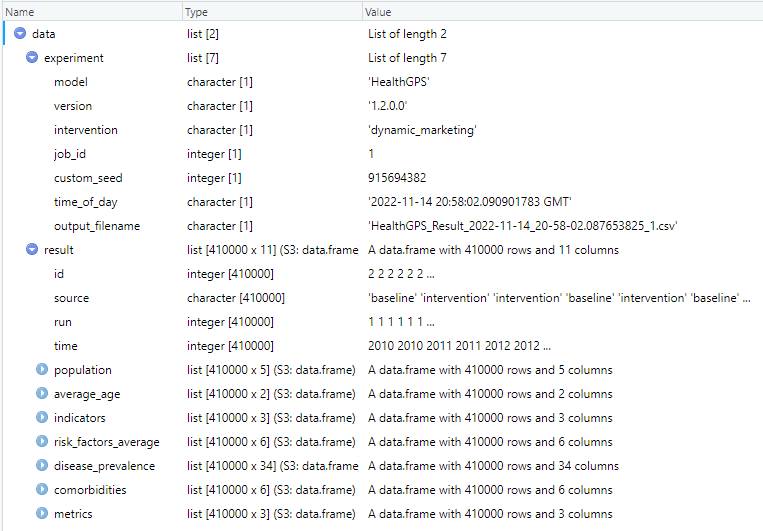
The above script reads the results data from file and makes the data variable available in R for analysis as shown below, it is equally easy to write a R structure to a JSON string or file.


Health-GPS results in R data frame example

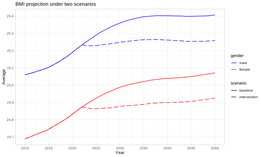
The results file contains the output of all simulations in the experiment, baseline, and intervention scenarios over one or more runs. The user should not assume data order during analysis of experiments with intervention scenarios, the results are published by both simulations running in parallel asynchronously via messages, the order in which the messages arrive at the destination queue, before being written to file is not guaranteed. A robust method to tabulate the results shown above, is to always group the data by: data.result(source, run, time), to ensure that the analysis algorithms work for both types of simulation experiments. For example, using the results data above in R, the following script will tabulate and plot the experiment’s BMI projection.

require(dplyr)
require(ggplot2)

# create groups frame
groups <- data.frame(data$result$source, data$result$run, data$result$time)
colnames(groups) <- c("scenario", "run", "time")

# create dataset
risk_factor <- "BMI"
sim_data <- cbind(groups, data$result$risk_factors_average[[risk_factor]])

# pivot data
info <- sim_data %>% group_by(scenario, time) %>%
  summarise(runs = n(),
            avg_male = mean(male, na.rm = TRUE),
            sd_male = sd(male, na.rm = TRUE),
            avg_female = mean(female, na.rm = TRUE),
            sd_female = sd(female, na.rm = TRUE),
            .groups = "keep")

# reshape data
df <- data.frame(scenario = info$scenario, time = info$time, runs = info$runs,
      bmi = c(info$avg_male, info$avg_female),
      sd = c(info$sd_male, info$sd_female),
      se = c(info$sd_male / sqrt(info$runs), info$sd_female) / sqrt(info$runs),
      gender = c(rep('male', nrow(info)), rep('female', nrow(info))))

# Plot BMI projection
p <- ggplot(data=df, aes(x=time, y=bmi, group=interaction(scenario, gender))) +
  geom_line(size=0.6, aes(linetype=scenario, color=gender)) + theme_light() +
  scale_linetype_manual(values=c("baseline"="solid","intervention"="longdash")) +
  scale_color_manual(values=c("male"="blue","female"="red")) +
  scale_x_continuous(breaks = pretty(df$time, n = 10)) +
  scale_y_continuous(breaks = pretty(df$bmi, n = 10)) +
  ggtitle(paste(risk_factor, " projection under two scenarios")) +
  xlab("Year") + ylab("Average")

show(p)


Experiment BMI projection example

In a similar manner, the resulting dataset df, can be re-created and expanded to summarise other variables of interest, create results tables and plots to better understand the experiment.

Topic	Document
User docs index	user/README.md
Full configuration & HPC	User Guide
Build from source	Developer Guide
Windows MSVC failures	MSVC troubleshooting
FINCH / Kevin Hall inputs	FINCH linear models guide
Technical docs	Technical documentation index
Documentation home	documentation/README.md

â† User documentation index · Documentation index

Author: Mahima Ghosh

Global Health Policy Simulation model

Quick Start

Example usage

Results

Analysing the JSON output data

Related documentation