Global Health Policy Simulation model

Introduction

Health-GPS is a modular and flexible microsimulation framework developed in collaboration between the Centre for Health Economics & Policy Innovation (CHEPI), Imperial College London; and INRAE, France. It was created for the STOP project and now supports analysis of health and economic impacts of policies on chronic diseases and obesity, including childhood obesity in European settings.

Health-GPS models the impacts of behavioural and metabolic risk factors on chronic diseases and measures lifelong outcomes so researchers can test the effectiveness of health policies and interventions. The framework has been extended for additional CHEPI-led work, including FINCH, GOLDFINCH, CoDiet, JACARDI, and JA PreventNCD. Project-specific inputs are maintained in HealthGPS-examples; the table below links each setting to a typical example folder.

Setting / project	More information	Example inputs (HealthGPS-examples)
STOP (France-style HLM)	STOP project	HLM_France
India	HFSS food tax modelling in India (CHEPI)	KevinHall_India
FINCH	FINCH (CHEPI)	KevinHall_FINCH
GOLDFINCH	GOLDFINCH (CHEPI)	Use inputs in progress
CoDiet	CoDiet (CHEPI)	Use inputs in progress
JACARDI	JACARDI (CHEPI)	Use inputs in progress
JA PreventNCD	JA PreventNCD (CHEPI)	Use inputs in progress

For FINCH-specific modelling (income, Kevin Hall, predictors), see the FINCH guide. For a full map of how every person attribute is assigned and updated, see How Health-GPS models a person.

Health-GPS creates a virtual population representative of a distinct country’s population and simulates close to reality life histories from birth to death of each member of the population including key characteristics such as gender, age, socio-economic status, risk factors, and disease profiles. These characteristics evolve over time and are updated in discrete time annually using statistical and probabilistic models which are calibrated to reproduce key demographic and epidemiological statistics from the specific country. The model uses proprietary equations to account for a variety of complex interactions such as risk factor-disease interactions and disease-disease interactions. Modellers are then able to evaluate health-related policies by changing some of the parameters and comparing the outputs with a baseline simulation. The model produces detailed quantitative outputs covering demographics, risk factors, diseases, mortality, global health estimates and health care expenditure, which could then be used to complement qualitative policy evaluation tools.

General Workflow

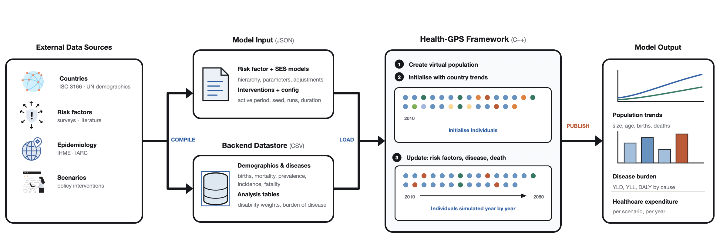
The Health-GPS workflow is summarised below, datasets from many disconnected sources are used to define the various modules and components of the framework. Commonly used datasets are processed, aggregated, indexed by country, and stored in the backend datastore, while research specific datasets are analysed externally to build the risk factors and socio-economic status modules, design and parameterise intervention to be tested.


Health-GPS General Workflow Diagram

The simulation creates the virtual population, simulates the synthetic individuals over time, collects population statistics and publish to the outside world at the end of each simulated time step. It is the user’s responsibility to analyse and quantify the model results, which are saved to a chosen output folder as JSON and CSV, and optionally income-stratum CSVs or individual ID tracking CSVs (same person IDs in baseline and intervention when tracking is enabled). See the User Guide - Results and Policy Evaluation below.

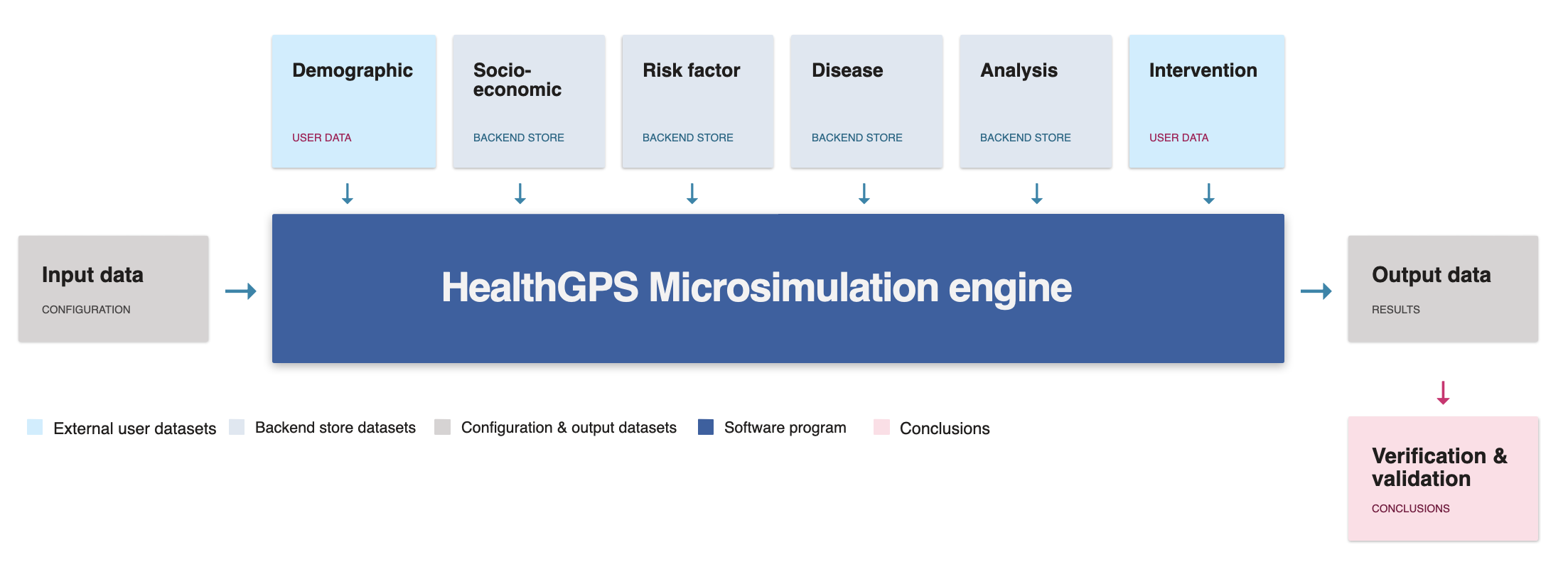
Health-GPS is a flexible and modular framework, written in modern C++, designed using object-oriented principles to provide the building blocks necessary to compose the overall microsimulation, several data sources, modules, and sub-model are required as shown below.


Health-GPS Concept Diagram

Modules Dynamic

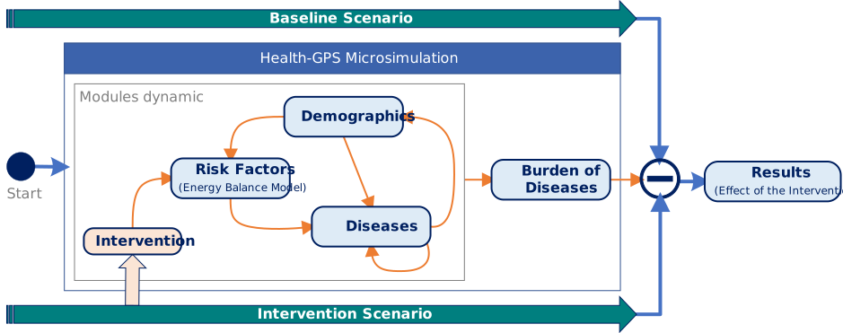
The framework defines multi-dimensional interactions on demographics, risk factors, diseases and intervention modules as shown below. The model dynamics capture the effects of the various interacting modules overtime to stablish the population baseline projection and quantify the impact of interventions on risk factors, the burden of diseases (BoD) module estimate population outcomes such as risk factors, disease prevalence, and health care expenditure. Finally, the different between the two scenarios is the effect of the intervention.


Health-GPS Dynamics Diagram

A brief overview of each module is provided next, the framework has been designed to allow module composition, modellers can experiment with different module implementations at run-time.

Demographics

The population historical trends and projections are used to define the baseline scenario for the model. The model requires historical and projected populations by year, age, and gender for each country of interest, covering the entire duration of the experiment. All data processing, units’ conversion, gap filling, smoothing, etc, must be carried out outside to produce the complete datasets required. The following demographic measures are required by the model:

Population size
Birth rates
Death rates
Residual Mortality - deaths from non-modelled causes.

Births, deaths, and immigration are the only drivers of changes in demographics in a population. While the births and deaths modelling are data driven, finding accurate data about immigration is more challenging. Net migration, the net flow of migrants between two consecutive years, is estimated as the difference by age and gender between the simulated population and the expected population from the country’s input data.

Socio-Economic Status (SES)

SES plays an important role in the levels of risk factors observed within the population. The levels of income and education can influence the nature of diet, and physical activity. In simple France-style configs, Health-GPS models SES as a continuous noise draw (ses) assigned at birth and held fixed. Income categories, quintile adjustment, and FINCH-style predictors are configured separately via project_requirements and modelling CSVs; see the FINCH guide and Software Architecture.

Risk Factors

The population cultural and social behaviours are represented by risk factors, defined as any attributes that can influence the likelihood of acquiring a disease. Individual choices such as smoking, alcohol consumption, physical activity, and diet, can lead to long-term consequences such as hypertension, obesity, and diabetes. Furthermore, certain diseases can be risk factors for other diseases or certain types of cancers.

The dynamics of risk factors modelling is a major challenge for health policy modellers, there are divergent opinions on the types and directions of causality between risk factors and diseases. Health-GPS defines a dynamic hierarchical risk factor model structure, modellers can configure the hierarchy outside for different problems, fit parameters to data and provide to fully built model as part of the experiment configuration.

Energy Balance Model (EBM)

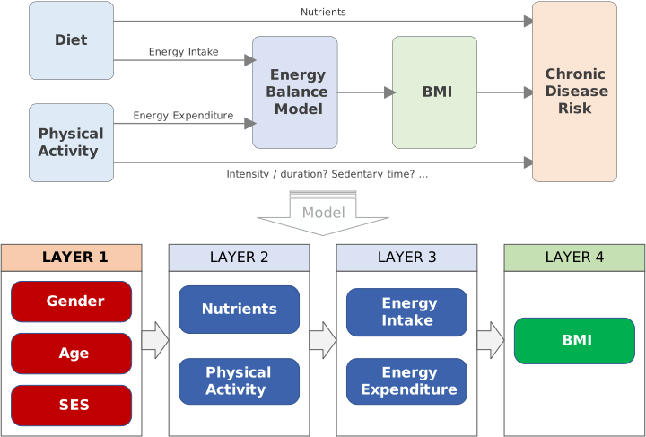
To represent childhood obesity, national dietary surveys from various European countries are analysed to build the risk factor model. Estimates of yearly changes in physical activity, diet, energy balance, and Body Mass Index (BMI) are created using dietary and anthropometric surveys. These include measures of physical activity expressed in metabolic equivalents (METs) and macronutrients intakes measures including grams of fat, carbohydrates, protein, fibre, salt, and sugar. The general concept for an EBM is shown below (top diagram), and a possible Health-GPS translation is provided for illustration purpose.


Energy balance model structure example

The calibration of the equations is carried out outside of the model by gender for children and adults separately to ensure capturing gender- and age-related differences. Emphasis is placed on capturing the rapid growth and changes in children BMIs. International anthropometric references are used to properly classify individuals as normal weight, overweight or obese. This classification is used throughout the simulation to identify children with growth problems and devise appropriate policies and interventions to tackle the health issues.

Diseases

Individuals may acquire new diseases for many reasons, including genetics, environment, and lifestyles. The associations between risk factors and the incidence of certain types of diseases is a major subject being widely study. Health-GPS accounts for the associations between risk factors and diseases by using equations to translate exposures to risk factors into probabilities that are used to simulate the incidence of diseases in the population.

The association between risk factor and disease stays constant throughout the simulation, however any changes in the distribution of a risk factor, will still translate to more/fewer disease cases through relative risk equations. Any change in the prevalence of a disease is therefore solely caused by changes in risk factors distributions alongside the ageing effect on the simulated population. Health-GPS supports two groups of diseases: general noncommunicable diseases, and types of cancer respectively.

Burden of Diseases

Collects statistical indicators about the simulated population, life expectancy, disease prevalence, risk factors exposure; and standardised metrics such as years of life lost due to premature mortality (YLL), years of healthy life lost due to disability (YLD), disability-adjusted life years (DALY), and healthcare expenditure (HCE) to reflect the impact of the intervention compared to a status-quo simulation.

Policy Evaluation

The overall approach adopted to evaluate the impacts and cost-effectiveness of intervention policies to reduce childhood obesity using the policy simulation tool is based upon “what-if” analyses to quantify the causal relations between variables, scenarios can be classified as:

Baseline scenarios: elaborated to define the trends in observed childhood obesity we measure outcomes against (e.g., population, calories intake, diseases prevalence trends).
Intervention scenarios: policies designed to change the observed trends in childhood obesity during a specific time frame (e.g., food labelling, healthy eating promotion, BMI reduction).

The choice of baseline scenario is critical for analyses as it serves as a reference for comparison and can influence outcomes. Having defined the baseline scenario, the simulation assesses the impacts of different intervention policies by projecting populations, risk factors, diseases, and life trajectories into the future comparing pairs of no-intervention and intervention scenarios.

The first run evaluates the no-intervention, “baseline scenario” where demographics, risk factors, and diseases are projected based solely on estimates from historical data. The second run evaluates the “intervention scenario” where a specific policy is applied to the same population with the aim of modifying the underlying trends and risk factor distribution.

Policy levers sequence

Policies are configured in running (scenario type, policy_start_year) and in modelling CSVs (for example FINCH policyeffect_model.csv / S*_policyeffect_model.csv). The same module stack runs in both scenarios. Only the intervention scenario evaluates policy equations after the start year, and only intervention may apply optional PIF to disease incidence.

sequenceDiagram
    autonumber
    participant Cfg as config.json + policy CSVs
    participant Host as Console host
    participant Scn as Intervention scenario
    participant RF as Risk-factor models
    participant Pers as Person state
    participant Dis as Disease models
    participant Ana as Analysis

    Cfg->>Host: running.policy_start_year, scenario type
    Cfg->>Host: Policy coefficient CSVs / scenario class
    Host->>Scn: Create Intervention Simulation

    Note over Scn,Ana: Years before policy_start_year
    loop Each year where time_now < policy_start_year
        Scn->>RF: Dynamic update without policy effect
        RF->>Pers: Update foods, PA, weight, BMI as usual
        Scn->>Dis: Incidence without PIF
        Scn->>Ana: Publish year (looks like baseline path)
    end

    Note over Scn,Ana: Policy window (time_now >= policy_start_year)
    loop Each year in the policy window
        Scn->>RF: Evaluate policy linear model on predictors
        Note right of RF: e.g. intercept + beta * log_income,<br/>log_EnergyIntake, gender2, region dummies
        RF->>Pers: Apply policy delta / trend to targeted risk factors
        Note right of Pers: clamp to configured ranges<br/>optional factors-mean re-alignment
        Scn->>Dis: Incidence with optional PIF
        Note right of Dis: P = incidence * RR / meanRR * (1 - PIF)
        Dis->>Pers: New active disease cases (or remissions)
        Scn->>Ana: Publish intervention year aggregates
    end

    Ana-->>Host: Intervention JSON / CSV / optional ID tracking

Policy sequence: before policy_start_year the intervention run follows the no-policy path; afterwards policy equations and optional PIF change risk factors and disease incidence. FINCH policy naming: FINCH guide.

Baseline and intervention paired run

When an intervention is configured, the Runner starts baseline and intervention simulations together (separate threads, separate Person populations). Synchronisation is one-way: baseline → intervention over a SyncChannel, and only aggregate tables are transferred (not individual people). Initial cohort person IDs match across scenarios (id = slot + 1) so optional ID tracking can compare the same starting individuals.

sequenceDiagram
    autonumber
    participant Host as Console / Runner
    participant Base as Baseline Simulation
    participant Chan as SyncChannel
    participant Intv as Intervention Simulation
    participant OutB as Baseline outputs
    participant OutI as Intervention outputs

    Host->>Base: Create Simulation baseline
    Host->>Intv: Create Simulation intervention
    Note over Base,Intv: Same config, datastore, seeds, population size<br/>Initial IDs 1..N match across scenarios

    par Initialise both populations
        Base->>Base: Demographics, SES, static+dynamic RF, diseases
        Intv->>Intv: Same init order (no policy yet if before start year)
    end

    loop Each simulated year
        Note over Base,Chan: Baseline computes shared aggregates
        Base->>Base: Demographic update (deaths, age++, births)
        Base->>Chan: Send ResidualMortalityMessage age x sex
        Base->>Base: Net immigration vs expected population
        Base->>Chan: Send NetImmigrationMessage age x sex
        Base->>Base: SES, RF update, diseases (no policy / no PIF)
        opt Factors-mean / Kevin Hall adjustments enabled
            Base->>Chan: Send adjustment tables (RF means / weight)
        end
        Base->>OutB: Publish ResultEventMessage (+ optional tracking)

        Note over Chan,Intv: Intervention receives aggregates, then applies policy
        Chan-->>Intv: Residual mortality table
        Chan-->>Intv: Net immigration table
        opt Adjustment sync present
            Chan-->>Intv: Factors-mean / Kevin Hall adjustment tables
        end
        Intv->>Intv: Demographic update using synced residual mortality
        Intv->>Intv: Apply synced net migration
        Intv->>Intv: SES, RF update
        alt time_now >= policy_start_year
            Intv->>Intv: Apply policy effects to risk factors
            Intv->>Intv: Disease update with optional PIF
        else before policy start
            Intv->>Intv: Disease update without PIF
        end
        Intv->>OutI: Publish ResultEventMessage (+ optional tracking)
    end

    Note over Host,OutI: What is NOT synced
    Note over Host,OutI: No Person objects, no IDs, no per-person region/ethnicity/RF copies

    Host->>Host: External comparison: intervention minus baseline<br/>BoD, risk-factor means, HCE, optional matched IDs

Paired baseline/intervention sequence: parallel runs, one-way aggregate sync on residual mortality, net immigration, and optional adjustment tables; policy and PIF only on the intervention side. See same-person ID plan.

Same person ID across baseline and intervention

For the initial cohort, Health-GPS assigns each synthetic person a stable person ID (derived from their slot in the population) so the same logical individual shares the same ID in both baseline and intervention runs. That makes it possible to compare scenarios at the person level - for example in optional tracking output - not only from aggregate JSON and CSV summaries. Life paths can still diverge after the intervention is applied; matching IDs mean “same starting person for comparison”, not guaranteed identical outcomes.

When you need filtered per-person time series (run, year, scenario, demographics, selected risk factors), enable output.individual_id_tracking in config. The model then writes an additional *_IndividualIDTracking.csv alongside the main results. Configuration, filters, and an example are in the User Guide - Output (FINCH example: KevinHall_FINCH/config.json in HealthGPS-examples). Design notes: same-person ID plan, individual ID tracking plan.

Finally, detailed analysis can be carried out, externally, to compare the two simulated scenarios results in terms of population demographics and burden of diseases to estimate the cost-effectiveness and impacts of the targeted intervention in tackling childhood obesity.

Simulation Workflow

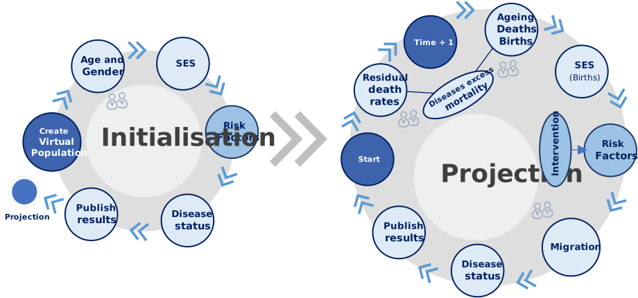
The microsimulation follows a two-step process to capture time-serial and cross-sectional correlations between risk factors, preserve the cross-sectional correlations between factors, and their hierarchical structure to allow changes to be propagated from lower to high level variables. The workflow consists of two main algorithms to initialise and project the virtual population over time respectively. Creating and initialising the virtual population is the first step of a simulation run, while the algorithm projecting the population over time is the core of the microsimulation as shown below.


Health-GPS Workflow Diagram

The diagram below is the whole-picture sequence for one experiment: load inputs, initialise every person, then advance year by year until the configured end time. Baseline and intervention use the same module order; only policy levers and optional PIF differ.

Risk-factor packs: config has two slots historically named static and dynamic. Those are pipeline roles (initialisation-oriented pack vs time-update-oriented pack), not labels for individual nutrients. Both slots run at init and again each year; see Models overview — static vs dynamic. Person-field maths: How Health-GPS models a person.

sequenceDiagram
    autonumber
    participant Host as Console host
    participant Sim as Simulation
    participant Demo as Demographics
    participant SES as SES
    participant RF as Risk factors
    participant Dis as Diseases
    participant Ana as Analysis
    participant Out as File outputs

    Note over Host,Out: Setup
    Host->>Sim: Load config, datastore, static/dynamic model packs
    Host->>Sim: Build baseline scenario (+ optional intervention)

    rect rgb(251, 229, 213)
        Note over Sim,Ana: Initialisation once per run
        Sim->>Demo: Assign age, gender, region, ethnicity
        Demo-->>Sim: Core demographics on each Person
        Sim->>SES: Draw ses from Normal(mu, sigma)
        Sim->>RF: Static generate then dynamic generate
        Note right of RF: Income, PA, foods/nutrients,<br/>height, weight, BMI as configured
        RF-->>Sim: risk_factors (+ PA / income fields)
        Sim->>Dis: Prevalence initialise from RR tables
        Sim->>Ana: Initial population statistics
    end

    loop Each year from start_time to end_time
        Note over Sim,Out: Yearly projection
        Sim->>Demo: Deaths, age + 1, births
        Sim->>Demo: Net migration in or out
        Sim->>SES: Redraw ses for newborns only
        Sim->>RF: Dynamic risk-factor update
        Sim->>Dis: Remission then incidence (+ optional PIF)
        Sim->>Ana: Publish year aggregates
        Ana->>Out: JSON summary, main CSV
        opt Income / ID tracking enabled
            Ana->>Out: Income-stratum CSVs and/or IndividualIDTracking.csv
        end
    end

    Note over Host,Out: Compare baseline vs intervention externally

Whole-picture Health-GPS sequence: setup, one-time initialisation, then the yearly module loop that writes analysis outputs.

The initialisation sets the simulation world clock, in years, to the user’s defined start time, and requests the simulation modules to initialise the relevant properties of the virtual population individuals. The projection moves the simulation clock, in years, forwards until the user’s defined end time is reached, at which point the algorithm terminates.

Data Sources

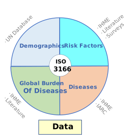
Health-GPS makes use of various types of data such as cross-sectional and longitudinal surveys to produce consistent estimates of a particular variable of interest. To reconcile large swathes of datasets describing determinants of health, demographics, socio-economic, behavioural, risk exposure, diseases, healthcare delivery and expenditure from otherwise unconnected sources, the Health-GPS data model adopts the ISO 3166 country code to link all datasets as shown below.


Health-GPS Data Reconciliation

The reconcile process can be extremely laborious with each dataset having to be processed individually to for general data cleansing, map country code, use consistent unit of measurement, filling gaps, and smoothing. Health-GPS assumes complete datasets, all data processing must take place out outside of the model.

Documentation map

All project docs live under documentation/. Start at README.md.


Health-GPS Documentation Guide

Folder	Audience	Contents
user/	Modellers, policy analysts	Quick Start, User Guide, Schemas, Models overview - user index
developer/	Software developers	Architecture, data model, build guide, Pages deploy troubleshooting, MSVC note, GitHub flow - developer index
technical/	Economists and developers	FINCH guide, simulation models reference, update reports, feature plans - technical index

Recommended starting points

New to Health-GPS -> Quick Start
FINCH / Kevin Hall inputs -> FINCH linear models guide
What changed in 2026 -> Update report
Threading and HPC sizing -> Performance guide
Building from source -> Developer Guide
Per-person baseline vs intervention output -> User Guide - Output
Config validation / $schema / v1 vs v2 -> Configuration schemas
Which model does what (HLM, Kevin Hall, …) -> Models overview
Windows build fails (cstdint / MSVCRTD.lib) -> MSVC troubleshooting
Pages deploy failed (Configure HealthGPS) -> Docs deploy troubleshooting
Documentation questions -> see Author at the bottom of each page (documentation index)

From	To
Documentation root	User / Developer / Technical
User index	Developer index / Technical index
Developer index	User index / MSVC note
Technical index	Developer Guide / User Guide

Author: Mahima Ghosh