Global Health Policy Simulation model

User Guide

The Health-GPS microsimulation is a data driven modelling framework, combining many disconnected data sources to support the various interacting modules during a typical simulation experiment run. The framework provides a pre-populated backend data storage to minimise the learning curve for simple use cases, however advance users are likely to need a more in-depth knowledge of the full modelling workflow. A high-level representation of the microsimulation user workflow is shown below, it is crucial for users to have a good appreciation for the general dataflows and processes to better design experiments, configure the tool, and quantify the results.


Health-GPS Workflow Diagram

As with any simulation model, the workflow starts with data, it is the user’s responsibility to process and analyse the input data, define the model’s hierarchy, fit parameters to data, and design intervention. A configuration file is used to provide the user’s datasets, model parameters, and control the simulation experiment runtime. The model is invoked via a Command Line Interface (CLI), which validates the configuration contents, loads associated files to create the model inputs, assembles the microsimulation with the required modules, evaluates the experiment, and writes the results to a chosen output file and folder. Likewise, it is the user’s responsibility to analyse and quantify the model results and draw conclusions on the cost-effectiveness of the intervention.

See Quick Start to get started using the microsimulation with a working example.

1.0 Configuration

The high-level structure of the configuration file used to create the model inputs, in JSON format, is shown below. The structure defines the schema version, the user’s dataset file, target country with respective virtual population settings, external models’ definition with respective fitted parameters, simulation experiment options including diseases selection, and intervention scenario, and finally the results output location.

{
    "version": 2,
    "inputs": {
        "dataset": {},
        "settings": {
            "country_code": "FRA",
            "size_fraction": 0.0001,
            "age_range": [ 0, 100 ]
        }
    },
    "modelling": {
        "ses_model": {},
        "risk_factors": [],
        "dynamic_risk_factor": "",
        "risk_factor_models": {},
        "baseline_adjustments": {}
    },
    "running": {
        "seed": [123456789],
        "start_time": 2010,
        "stop_time": 2050,
        "trial_runs": 1,
        "sync_timeout_ms": 15000,
        "diseases": ["alzheimer","asthma","colorectalcancer","diabetes","lowbackpain","osteoarthritisknee"],
        "interventions": {
            "active_type_id": "",
            "types": {}
        }
    },
    "output": {
        "comorbidities": 5,
        "folder": "${HOME}/healthgps/results/france",
        "file_name": "HealthGPS_Result_{TIMESTAMP}.json"
    }
}

1.1 Inputs

The inputs section sets the target country information, the file sub-section provides details of data used to fit the model, including file name, format, and variable data type mapping with the model internal types: string, integer, float, double. The user’s data is required only to provide a visual validation of the initial virtual population created by the model, this feature should be made optional in the future, the following example illustrates the data file definition:

...
"inputs": {
    "dataset": {
        "name": "France.DataFile.csv",
        "format": "csv",
        "delimiter": ",",
        "encoding": "ASCII",
        "columns": {
            "Year": "integer",
            "Gender": "integer",
            "Age": "integer",
            "Age2": "integer",
            "Age3": "integer",
            "SES": "double",
            "PA": "double",
            "Protein": "double",
            "Sodium": "double",
            "Fat": "double",
            "Energy": "double",
            "BMI": "double"
        }
    }
}
...

1.2 Modelling

The modelling section, defines the SES model, and the risk factor model with factors identifiers, hierarchy level, data range and mapping with the model’s virtual individual properties (proxy). The risk_factor_models sub-section provides the fitted parameters file, JSON format, for each hierarchical model type, the dynamic risk factor, if exists, can be identified by the respective property. Finally, the baseline adjustments sub-section provides the adjustment files for each hierarchical model type and gender.

...
"modelling": {
    "ses_model": {
        "function_name":"normal",
        "function_parameters":[0.0, 1.0]
    },
    "risk_factors": [
        {"name":"Gender",   "level":0, "proxy":"gender", "range":[0,1]},
        {"name":"Age",      "level":0, "proxy":"age",    "range":[1,87]},
        {"name":"Age2",     "level":0, "proxy":"",       "range":[1,7569]},
        {"name":"Age3",     "level":0, "proxy":"",       "range":[1,658503]},
        {"name":"SES",      "level":0, "proxy":"ses",    "range":[-2.316299,2.296689]},
        {"name":"Sodium",   "level":1, "proxy":"",       "range":[1.127384,8.656519]},
        {"name":"Protein",  "level":1, "proxy":"",       "range":[43.50682,238.4145]},
        {"name":"Fat",      "level":1, "proxy":"",       "range":[45.04756,382.664]},
        {"name":"PA",       "level":2, "proxy":"",       "range":[22.22314,9765.512]},
        {"name":"Energy",   "level":2, "proxy":"",       "range":[1326.14051,7522.496]},
        {"name":"BMI",      "level":3, "proxy":"",       "range":[13.88,39.48983]}
    ],
    "dynamic_risk_factor": "",
    "risk_factor_models": {
        "static": "France_HLM.json",
        "dynamic": "France_EBHLM.json"
    },
    "baseline_adjustments": {
        "format": "csv",
        "delimiter": ",",
        "encoding": "UTF8",
        "file_names": {
            "factors_mean_male":"France.FactorsMean.Male.csv",
            "factors_mean_female":"France.FactorsMean.Female.csv"
        }
    }
}
...

The risk factor model and baseline adjustment files have their own schemas and formats requirements, these files structure are defined separately below, after all the configuration file sections.

1.3 Running

The running section defines simulation run-time period, start/stop time respectively in years, pseudorandom generator seed for reproducibility or empty for auto seeding, the number of trials to run for the experiment, and scenarios data synchronisation timeout in milliseconds. The model supports a dynamic list of diseases in the backend storage, the diseases array contains the selected disease identifiers to include in the experiment. The interventions sub-section defines zero or more interventions types, however, only one intervention at most can be active per configuration, the active_type_id property identifies the active intervention, leave it empty for a baseline scenario only experiment.

...
"running": {
    "seed": [123456789],
    "start_time": 2010,
    "stop_time": 2050,
    "trial_runs": 1,
    "sync_timeout_ms": 15000,
    "diseases": ["alzheimer", "asthma", "colorectalcancer", "diabetes", "lowbackpain", "osteoarthritisknee"],
    "interventions": {
        "active_type_id": "dynamic_marketing",
        "types": {
            "simple": {
                "active_period": {
                    "start_time": 2021,
                    "finish_time": 2021
                },
                "impact_type": "absolute",
                "impacts": [
                    { "risk_factor":"BMI", "impact_value": -1.0, "from_age":0, "to_age":null}
                ]
            },
            "dynamic_marketing": {
                "active_period": {
                    "start_time": 2022,
                    "finish_time": 2050
                },
                "dynamics":[0.15, 0.0, 0.0], 
                "impacts": [
                    {"risk_factor":"BMI", "impact_value":-0.12, "from_age":5,  "to_age":12},
                    {"risk_factor":"BMI", "impact_value":-0.31, "from_age":13, "to_age":18},
                    {"risk_factor":"BMI", "impact_value":-0.16, "from_age":19, "to_age":null}
                ]
            },
            "physical_activity": {
                "active_period": {
                    "start_time": 2022,
                    "finish_time": 2050
                },
                "coverage_rates": [0.90],
                "impacts": [
                    {"risk_factor":"BMI", "impact_value":-0.16, "from_age":6,  "to_age":15},
                    {"risk_factor":"BMI", "impact_value":-0.08, "from_age":16,  "to_age":null}
                ]
            },
            ...
        }
    }
}
...

Unlike the diseases data driven definition, interventions can have specific data requirements, rules for selecting the target population to intervening, intervention period transition, etc, consequently the definition usually require supporting code implementation. Health-GPS provides an interface abstraction for implementing new interventions and easily use at runtime, however the implementation must also handle the required input data.

1.4 Output

Finally, output section repeated below, defines the maximum number of comorbidities to include in the results, and the output folder and file name. The configuration parser can handle folder name with environment variables such as HOME on Linux shown below, however care must be taken when running the model cross-platform with same configuration file. Likewise, file name can have a TIMESTAMP token, to enable multiple experiments to write results to the same folder on disk without file name crashing.

...
"output": {
    "comorbidities": 5,
    "folder": "${HOME}/healthgps/results/france",
    "file_name": "HealthGPS_Result_{TIMESTAMP}.json"
}
...

The file name can have a job_id, passed as a CLI parameter, added to the end when running the simulation in batch mode, e.g., HPC cluster array. This feature enables the batch output files to be collated together to produce the complete results dataset for analysis.

1.5 Risk Factor Models

Health-GPS requires two types of risk factor models to be externally created by the user, fitted to data, and provided via configuration: static and dynamic respective. The first type is used to initialise the virtual population with the current risk factor trends, the second type is used to update the population attributes, accounting for the dynamics of the risk factors as time progresses in the simulation and individual’s age.

The risk factor models definition adopts a semi-parametric approach based on a regression models with sampling from the residuals to conserve the original data distributions. Each risk factor model file contains the various fitted regression models’ coefficients, residuals, and other related values, that must be provided in a consistent format independent of the fitting tool.

1.5.1 Static

Initialise the virtual population, created by the model, with risk factor trends like the real population in terms of statistical distributions of the modelled variables. In addition to the regression fitted values, the static model includes transition matrix, inverse transition matrix, and independent residuals for sampling to conserve the correlations.

The structure of a static model file is shown below, the size of the fitted residuals, arrays/matrices, are data size dependent, therefore this model type does not scale well with datasets size, N, and can potentially result in excessive memory usage.

{
    "models": {
        "Sodium": {
            "formula": "...",
            "coefficients": {
                "Intercept": {
                    "value": 2.0303445114896066,
                    "stdError": 0.023969233176537191,
                    "tValue": 84.706277273694923,
                    "pValue": 0
                },
                "Gender": {..},
                "Age": {...},
                "Age2": {...},
                "Age3": {...},
                "SES": {...}
            },
            "residuals": [N],
            "fittedValues": [N],
            "residualsStandardDeviation": 1.4648008146487799,
            "rSquared": 0.13385827201094316
        },
        "Protein": {...},
        "Fat": {...},
        "PA": {...},
        "Energy": {...},
        "BMI": {...}
    },
    "levels": {
        "1": {
            "variables": ["Sodium", "Protein", "Fat"],
            "s": {
                "rows": N,
                "cols": 3,
                "data": [rows*cols]
            },
            "w": {
                "rows": 3,
                "cols": 3,
                "data": [rows*cols]
            },
            "m": {
                "rows": 3,
                "cols": 3,
                "data": [rows*cols]
            },
            "variances": [
                0.6027296236467885,
                0.30583191687945821,
                0.091438459473747832
            ],
            "correlation": {
                "rows": 3,
                "cols": 3,
                "data": [rows*cols]
            }
        },
        "2": {
            "variables": ["PA", "Energy"],
            ...
        },
        "3": {
            "variables": ["BMI"],
            ...,
            "correlation": {
                "rows": 1,
                "cols": 1,
                "data": [1.0]
            }
        },
    }
}

The file structure has been defined for completeness, not all values are used by the current model, for example, the coefficients goodness of fit (GoF) values, however, these values are negligible when compared with the large arrays and matrices of size N. The levels matrices calculated using Independent Component Analysis (ICA). are stored using row-major order, m is the transition matrix, w the inverse transition matrix, and s the independent residuals distribution for variables at each level.

1.5.2 Dynamic

Having initialised the virtual population risk factors, the dynamic model projects individuals’ risk factors over time using delta changes to current values. The structure of a dynamic model file is shown below, only the factors variable range, regression coefficients and residuals standard deviation are required, this model type definition is lite and can scale to any size datasets.

The first two properties document the model’s target country, and the percentage value used to calculate the risk factors variables range quartile from the respective dataset variables. The risk factors section defines the model hierarchy and must be copied into the configuration file, the factors range are used to constrain updates to the respective factors value at runtime.

{
    "Country": {"Code":250,"Name":"France","Alpha2":"FR","Alpha3":"FRA"},
    "BoundaryPercentage": 0.05,
    "RiskFactors": [
        {"Name":"Gender", "Level":0, "Proxy":"gender", "Range":[0, 1]},
        {"Name":"Age",    "Level":0, "Proxy":"age",    "Range":[1, 87]},
        {"Name":"Age2",   "Level":0, "Proxy":"",       "Range":[1, 7569]},
        {"Name":"Age3",   "Level":0, "Proxy":"",       "Range":[1, 658503]},
        {"Name":"SES",    "Level":0, "Proxy":"ses",    "Range":[-2.314, 2.310]},
        {"Name":"Sodium", "Level":1, "Proxy":"",       "Range":[1.146, 8.675]},
        {"Name":"Protein","Level":1, "Proxy":"",       "Range":[42.092, 238.414]},
        {"Name":"Fat",    "Level":1, "Proxy":"",       "Range":[44.781, 381.666]},
        {"Name":"PA",     "Level":2, "Proxy":"",       "Range":[400.0, 9769.837]},
        {"Name":"Energy", "Level":2, "Proxy":"",       "Range":[1315.532, 7545.832]}
        {"Name":"BMI",    "Level":3, "Proxy":"",       "Range":[13.532, 45.265]}
    ],
    "Variables": [
        {"Name":"dPA",     "Level":3, "Factor":"pa"},
        {"Name":"dEnergy", "Level":3, "Factor":"energy"},
        {"Name":"dProtein","Level":2, "Factor":"protein"},
        {"Name":"dSodium", "Level":2, "Factor":"sodium"},
        {"Name":"dFat",    "Level":2, "Factor":"fat"}
    ],
    "Equations": {
        "0-19": {
            "Female": [
                {
                    "Name": "BMI",
                    "Coefficients": {
                        "Intercept": -0.227646964586474,
                        "SES": -0.0201431467562394,
                        "Age": 0.0877002551156606,
                        "dPA": -4.63919783505021E-05,
                        "dEnergy": 0.00244125012762089
                    },
                    "ResidualsStandardDeviation": 1.2335501015137833
                },
                ...
            ],
            "Male": [
                ...,
                {
                    "Name": "Sodium",
                    "Coefficients": {
                        "Intercept": 0.0634502820168143,
                        "SES": 0.00549710735696626,
                        "Age": 0.0100775034506456
                    },
                    "ResidualsStandardDeviation": 0.2825432918724497
                }
            ]
        },
        "20-100": {
            "Female": [...],
            "Male": [...],
        }
    }
}

Variables are internal delta terms in the regression equations associated with specific factors at each hierarchical level. The order of the risk factors definition in the file is not important, the model is assembled dynamically using the level value in the risk factors hierarchy.

The equations section contains the model’s definition by age group and gender. The number of age group models is dynamic, the only constraint is that age groups must cover the age range required in the configuration file without any internal overlap.

1.5.3 Baseline Adjustments

To manage unknown trends in risk factors affecting the choices of baseline scenario, users can define adjustments values to keep the distributions of risk factors by gender and age constant over time. Separated files are defined, in comma separated format (CSV), for each combination of model type and gender, the adjustment files content must cove the age range required by the configuration settings. The structure and contents of an adjustment file is illustrated below.

Age,Sodium,Protein,Fat,PA,Energy,BMI
0,0.682,21.186,31.285,-158.128,169.349,2.922
1,0.544,17.733,26.261,-119.174,152.908,2.263
...
50,-0.105,-5.150,-7.019,57.353,-92.973,-0.564
51,-0.092,-4.780,-6.429,49.482,-88.769,-0.509
...
99,-0.593,-35.578,-66.544,-561.144,-141.747,-8.306
100,-0.658,-40.064,-74.064,-602.356,-145.923,-9.331

The values in the adjustment files are added to the model values, therefore a zero-adjustment value can be used to disable baseline adjustments for a specific risk factor variable.

2.0 Backend Storage

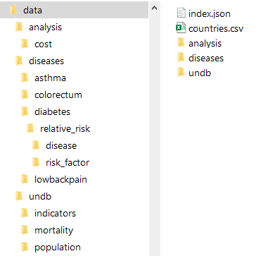
Health-GPS by default uses a file-based backend storage, which implements the Data Model to provides a reusable, reference dataset using a standardised format for improved usability, the dataset can easily be expanded with new data without code changes. The contents of the file-based storage is defined using the index.json file, which must live at the root of the storage’s folder structure as shown below.


File-based Backend Datastore example

The index file defines schema version, data groups, physical storage folders relative to the root folder, file names pattern, and stores metadata to identify the data sources, licences, and data limits for consistency validation. The data is indexed and stored by country files taking advantage of the model’s workflow, this minimises data reading time and enables the storage to scale with many countries.

The data model defines many data hierarchies, which have been flatten for file-based storage, file names are defined for consistency, avoid naming clashes, and ultimately to store processed data for machines consumption, not necessarily for humans. The high-level structure of the file-based storage index file, in JSON format, is shown below.

{
    "version": 2,
    "country": {
        "format": "csv",
        "delimiter": ",",
        "encoding": "UTF8",
        "description": "ISO 3166-1 country codes.",
        "source": "International Organization for Standardization",
        "url": "https://www.iso.org/iso-3166-country-codes.html",
        "license": "N/A",
        "path": "",
        "file_name": "countries.csv"
    },
    "demographic": {},
    "diseases": {
        "disease": {
            "relative_risk":{ },
            "parameters":{ },
        },
        "registry":[ ]
    },
    "analysis":{ }
}

The country data file lives at the root of the folder structure as shown above, therefore the path is left empty, and respective file name provided. The metadata is used only for documentation purpose, current Data API contracts have no support for surfacing metadata, therefore the metadata contents will be removed from the following sections for brevity and clarity.

The path and file_name properties are required and must be defined, all paths are relative to the parent folder.

The file store definition make use of tokenisation to represent dynamic contents in folders and files name. Tokens are substituted by their respective values in the file storage contents, for example, tokens {COUNTRY_CODE} and {GENDER} represent a country unique identifier and the gender value respectively. At runtime, tokens maps back to the storage’s folders and files name when replaced by the Data API calls parameters, dynamically reconstructing paths and files name.

2.1 Demographic

Defines the file storage for country specific data containing historic estimates and projections for various demographics measures by time, age and gender. The datasets limits for age and time variables are stored for validation, the projections property marks the starting point, in time, for projected values. Data files are stored in separated folders for population, mortality and demographic indicators respectively as shown below, file names must include the country’s unique identifier in place of the COUNTRY_CODE token.

...
"demographic": {
    "format": "csv",
    "delimiter": ",",
    "encoding": "UTF8",    
    ...
    "path": "undb",
    "age_limits": [0, 100],
    "time_limits": [1950, 2100],
    "projections": 2022,
    "population": {
        "description": "Total population by sex, annually from 1950 to 2100.",
        "path": "population",
        "file_name": "P{COUNTRY_CODE}.csv"
    },
    "mortality": {
        "description": "Number of deaths by age and gender.",
        "path": "mortality",
        "file_name": "M{COUNTRY_CODE}.csv"
    },
    "indicators": {
        "description": "Several indicators, e.g. births, deaths and life expectancy.",
        "path": "indicators",
        "file_name": "Pi{COUNTRY_CODE}.csv"
    }
}
...

2.2 Diseases

Defines the file storage for country specific data containing cross-sectional estimates by age and gender for various diseases measures, disease relative risk to other diseases, risk factor relative risk to diseases, and cancer parameters. Each disease is defined in a separate folder named using the disease identifier in place of the {DISEASE_TYPE} token, estimates for disease incidence, prevalence, mortality and remission are stored in a single file per country, files name must include the country’s unique identifier in place of the COUNTRY_CODE token as shown below. Cancer parameters are stored with same files name per country.

The relative risk data is stored in a sub-folder, with disease to disease interaction files defined in one folder and risk factor relative risk to diseases in another folder. The disease relative risk to diseases folder should contain data files for diseases with real interaction, when no file exists, the default value is used automatically. Similarly, the risk factor relative risk folder should only have files for risk factors with direct effect on the disease. In summary, only files with real relative risk values should be included.

...
"diseases": {
    "format": "csv",
    "delimiter": ",",
    "encoding": "UTF8",    
    ...
    "path": "diseases",
    "age_limits": [1, 100],
    "time_year": 2019,
    "disease": {
        "path": "{DISEASE_TYPE}",
        "file_name": "D{COUNTRY_CODE}.csv",
        "relative_risk":{
            "path": "relative_risk",
            "to_disease":{
                "path":"disease",
                "file_name": "{DISEASE_TYPE}_{DISEASE_TYPE}.csv",
                "default_value": 1.0
            },
            "to_risk_factor":{
                "path":"risk_factor",
                "file_name": "{GENDER}_{DISEASE_TYPE}_{RISK_FACTOR}.csv"
            }
        },
        "parameters":{
            "path":"P{COUNTRY_CODE}",
            "files":{
                "distribution": "prevalence_distribution.csv",
                "survival_rate": "survival_rate_parameters.csv",
                "death_weight": "death_weights.csv"
            }
        }
    },
    "registry":[
        {"group": "other", "id": "asthma", "name": "Asthma"},
        {"group": "other", "id": "diabetes", "name": "Diabetes mellitus"},
        {"group": "other",  "id": "lowbackpain", "name": "Low back pain"},
        {"group": "cancer", "id": "colorectum", "name": "Colorectum  cancer"}
    ]
}
...

The registry contains the dynamic list of disease types supported by the model. Diseases must belong to one pre-defined group, the id property is the disease unique identifier, and must have a display name.

To add a new disease to the storage:

Register the disease with a unique identifier, id
Create a folder named id inside the diseases folder
Populate the disease folder with the disease definition files

The disease id value now can be used in the configuration file to select diseases to include in a given simulation experiment.

2.3 Analysis

Defines the file storage for disease cost analysis for country specific data containing cross-sectional estimates by age for burden of disease measures. The datasets limit for the age variable is stored for validation, the time_year property identifies the cross-sectional data point for documentation purpose. The disability weights file provides global values for the disease analysis for all countries.

...
"analysis":{
    ...
    "path": "analysis",
    "age_limits": [1, 100],
    "time_year": 2019,
    "disability_file_name": "disability_weights.csv",
    "lms_file_name":"lms_parameters.csv",
    "cost_of_disease": {
        "path":"cost",
        "file_name": "BoD{COUNTRY_CODE}.csv"
    }
}
...

4.0 Running

Health-GPS has been designed to be portable, producing stable, and comparable results cross-platform. Only minor and insignificant rounding errors should be noticeable, these errors are attributed to the C++ application binary interface (ABI), which is not guaranteed to compatible between two binary programs cross-platform, or even on same platform when using different versions of the C++ standard library.

The code repository provides x64 binaries for Windows and Linux Operating Systems (OS), unfortunately, these binaries have been created using tools and libraries specific to each platform, and consequently have very different runtime requirements. The following step by step guide illustrates how to run the Health-GPS application on each platform using the include example model and reference dataset.

Windows OS

You may need to install the latest Visual C++ Redistributable on the machine, the application requires the 2022 x64 version to be installed.

Download the latest release source code and binaries for Windows from the repository.
Unzip both files content into a local directory of your choice (xxx).
Open a command terminal, e.g. Windows Terminal, and navigate to the directory used in step 2 (xxx).
Rename the data source subfolder (healthgps) by removing the version from folder’s name.
Run: X:\xxx> .\HealthGPS.Console.exe -f healthgps/example/France.Config.json -s healthgps/data where -f gives the configuration file full-name and -s the path to the root folder of the backend storage respectively.
The default output folder is C:/healthgps/results/france, but this can be changed in the configuration file (France.Config.json).

Linux OS

You may need to install the latest GCC Compiler and Intel TBB runtime libraries in your system, the application requires GCC 11.1 and TBB 2018 or newer versions to be installed.

Download the latest release source code and binaries for Linux from the repository.
Unzip both files content into a local directory of your choice (xxx).
Open a command terminal and navigate to the directory used in step 2 (xxx).
Rename the data source subfolder (healthgps) by removing the version from folder’s name.
Run: user@machine:~/xxx$ ./HealthGPS.Console.exe -f healthgps/example/France.Config.json -s healthgps/data where -f gives the configuration file full-name and -s the path to the root folder of the backend storage respectively.
The default output folder is $HOME/healthgps/results/france, but this can be changed in the configuration file (France.Config.json).

See Quick Start for details on the example dataset and known issues.

The included model and dataset provide an complete exemplar of the files and procedures described in this document. Users should use this exemplar as a starting point when creating production environments to aid the design and testing of intervention policies.

4.1 Results

The model results file structure is composed of two parts: experiment metadata and result array respectively, each entry in the result array contains the results of a complete simulation run for a scenario as shown below. The simulation results are unique identified the source scenario, run number and time for each result row, the id property identifies the message type within the message bus implementation. The model also output a detailed results file in Comma Separated Values (.csv), this associated output file name is included in the global summary file as shown below.

{
    "experiment": {
        "model": "HealthGPS",
        "version": "1.2.0.0",
        "intervention": "dynamic_marketing",
        "job_id": 0,
        "custom_seed": 123456789,
        "time_of_day": "2022-07-04 17:50:37.5678259 GMT Summer Time",
        "output_filename": "HealthGPS_Result_{TIME_STAMP}.csv"
    },
    "result": [
        {
            "id": 2,
            "source": "baseline",
            "run": 1,
            "time": 2010,
            ...
        },
        {
            "id": 2,
            "source": "intervention",
            "run": 1,
            "time": 2010,
            ...
        },
        ...
    ]
}

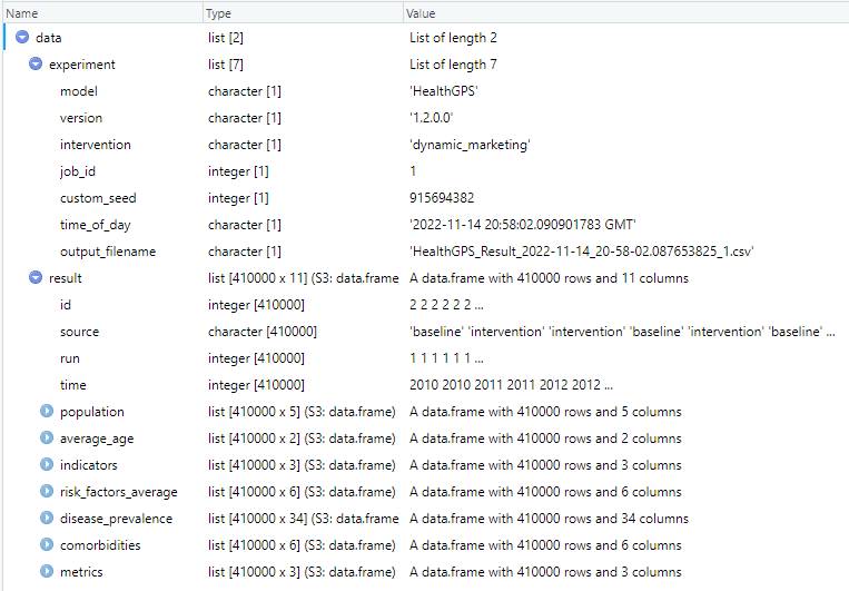
The content of each message is implementation dependent, JSON (JavaScript Object Notation), an open standard file format designed for data interchange in human-readable text, can represent complex data structures. It is language-independent; however, all programming language and major data science tools supports JSON format because they have libraries and functions to read/write JSON structures. To read the model results in R, for example, you need the jsonlite package:

require(jsonlite)
data <- fromJSON(result_filename.json)
View(data)

The above script reads the results data from file and makes the data variable available in R for analysis as shown below, it is equally easy to write a R structure to a JSON string or file.


Health-GPS results in R data frame example

The results file contains the output of all simulations in the experiment, baseline, and intervention scenarios over one or more runs. The user should not assume data order during analysis of experiments with intervention scenarios, the results are published by both simulations running in parallel asynchronously via messages, the order in which the messages arrive at the destination queue, before being written to file is not guaranteed. A robust method to tabulate the results shown above, is to always group the data by: data.result(source, run, time), to ensure that the analysis algorithms work for both types of simulation experiments. For example, using the results data above in R, the following script will tabulate and plot the experiment’s BMI projection.

require(dplyr)
require(ggplot2)

# create groups frame
groups <- data.frame(data$result$source, data$result$run, data$result$time)
colnames(groups) <- c("scenario", "run", "time")

# create dataset
risk_factor <- "BMI"
sim_data <- cbind(groups, data$result$risk_factors_average[[risk_factor]])

# pivot dataset
info <- sim_data %>% group_by(scenario, time) %>% 
  summarise(runs = n(),
            avg_male = mean(male, na.rm = TRUE),
            sd_male = sd(male, na.rm = TRUE),
            avg_female = mean(female, na.rm = TRUE),
            sd_female = sd(female, na.rm = TRUE),
            .groups = "keep")

# reshape dataset
df <- data.frame(scenario = info$scenario, time = info$time, runs = info$runs,
      bmi = c(info$avg_male, info$avg_female),
      sd = c(info$sd_male, info$sd_female),
      se = c(info$sd_male / sqrt(info$runs), info$sd_female) / sqrt(info$runs),
      gender = c(rep('male', nrow(info)), rep('female', nrow(info))))

# Plot BMI projection
p <- ggplot(data=df, aes(x=time, y=bmi, group=interaction(scenario, gender))) +
  geom_line(size=0.6, aes(linetype=scenario, color=gender)) + theme_light() +
  scale_linetype_manual(values=c("baseline"="solid","intervention"="longdash")) +
  scale_color_manual(values=c("male"="blue","female"="red")) +
  scale_x_continuous(breaks = pretty(df$time, n = 10)) +
  scale_y_continuous(breaks = pretty(df$bmi, n = 10)) +
  ggtitle(paste(risk_factor, " projection under two scenarios")) +
  xlab("Year") + ylab("Average")

show(p)


Experiment BMI projection example

In a similar manner, the resulting dataset df, can be re-created and expanded to summarise other variables of interest, create results tables and plots to better understand the experiment.

4.1.1 Detailed Results

The simulation detailed results file contains a dynamic number of columns, which depends on the risk factor model definition and diseases selection. The file’s data is grouped by sex and age, each row in the file can be unique identified by the following columns:

source - the simulation scenario: baseline or intervention.
run - the simulation run number, e.g., 1, 5, 50,
time - the simulation clock time, e.g., 2010, 2023, 2050.
gender_name - the sex group identifier: male or female.
index_id - the age group identifier, e.g., 0, 30, 70, 100.

The column count gives the number of individuals in the row group, the remaining columns contain average values for the group’s data at each column. This result file can easily be used to construct pivot tables and plots. The column count can be combined with the averaged columns to estimate other statistical measures, such as variance and standard deviation.

5.0 HPC Running

Although Health-GPS is compatible with most High Performance Computing (HPC) system, this section contents are specific for using Health-GPS software at the Imperial College London HPC system, which users need to register to get access and support. This HPC is Linux based, therefore users must be familiar with Unix command line and shell script to properly navigate the file system, run programs, and automate repetitive tasks.

Every software package installed in the HPC is called a module. The module system for centrally installed packages, must be used to find, load and unload installed modules and dependencies required to use a software package. The following module commands are essential to get started with Imperial HPC system:

Command	Description
module avail	List all modules available
module avail tools	Find all available versions of a software module
module add tools/dev	Load a module to be used into the job or user own space
module list	List all loaded modules
module rm tools/dev	Remove a loaded module version
module purge	Unload all loaded modules, clear all modules

Warning
Modules name are case sensitive for both script and search.

Module packages can be installed globally within the HPC system, old style, or different stacks depending on Software maturity and quality (recommended). To see all available stacks, type command: module av tools, the Health-GPS Software can be installed via three stacks:

local (tools/eb-dev) - installed locally in the user space, software development projects.
development (tools/dev) - a generic stack available on the login nodes but without any guarantees, software can change on short notice.
production (tools/prod) - a generic stack for software built to support specific architectures, and not available on the login nodes, only via job scripts. To view which software is installed, load the ‘tools/prod-headnode’ and search for the software.

Furthermore, the Portable Batch System (PBS), a batch job and computer system resource management package, is used by the Imperial HPC for job scheduling and users also need learn the PBS commands. A list of useful PBS commands used to submit, monitor, modify, and delete jobs can be found below:

Command	Action	Example	Description
qsub	Submit	qsub myjob	Submits the job “myjob” for the execution
qstat	Monitor	qstat	Show the status of all the jobs
’ ‘	’ ‘	qstat job_id	Show the status of single job
qalter	Modify	qalter -l ncpus = 4 job_id	Changes the attributes of the job
qdel	Delete	qdel job_id	Deletes the job with job id = job_id

An introduction to the PBS is beyond this tutorial, users are encouraged to attend dedicated courses provided by Imperial’s professional development programme to familiarise themselves with the HPC system and usage guidelines. This tutorial provides the basic steps required for finding, loading, and using installed Health-GPS software within the Imperial HPC system.

A job script using PBS comprises of three parts:

job parameters - resource allocation and job duration using BPS options.
required software - load required software modules to execute the application.
user command - execute the user application with given arguments.

The following job script (healthgps.pbs) executes Health-GPS version X.Y.Z.B on the development example and writes the console output to text file: healthgps.pbs.txt. The -GCCcore-11.3.0 part of the version name refers to the compiler toolset used to build the Health-GPS software and install on the HPC as described in the Developer Guide, this guide concerns only the use of installed modules.

#PBS -l walltime=00:30:00
#PBS -l select=1:ncpus=8:mem=64gb

cd $PBS_O_WORKDIR

module add tools/dev
module add Health-GPS/X.Y.Z.B-GCCcore-11.3.0

HealthGPS.Console -f healthgps/example/France.Config.json -s healthgps/data > healthgps.pbs.txt

To submit the above job script, check its status, and view the console output, the following PBS commands can be used:

# Submit Health-GPS job, print out the job id
qsub healthgps.pbs

# Check the status of all submitted jobs (not completed only). 
qstat

# View Health-GPS console output
cat healthgps.pbs.txt

Every job produces two log files, by default alongside the submitted job script, in this example:

healthgps.pbs.ejob_id - error messages (stderr)
healthgps.pbs.ojob_id - screen outputs and resource management messages (stdout)

Environment variable: $PBS_O_WORKDIR points to the submit directory and will exist while the job is running. This is where you submitted your job, usually a directory where your job script resides, and this variable can be used in a job script. The console output log file (healthgps.pbs.txt) is optional, it can be very useful when diagnosing Health-GPS configuration problem. This file also provides detailed simulation run-time information that can be harvested to quantify performance.

5.1 Array job script

The above example runs a single Health-GPS configuration, like a desktop computer (sequential), however, to run experiments with thousands of simulations, parallelisation is required, and HPC system when used effectively, can make a huge difference. One way of parallelising Health-GPS experiments using Imperial HPC is to use array job instead of single job per script, this breaks down a large experiment into small batches to be evaluated as parallel jobs.

To illustrate this mechanism, lets modify the job script above, and schedule 5 simulation batches using Health-GPS on the HPC to be evaluated in parallel.

#PBS -l walltime=01:00:00
#PBS -l select=1:ncpus=8:mem=64gb
#PBS -J 1-5

cd $PBS_O_WORKDIR

module add tools/dev
module add Health-GPS/X.Y.Z.B-GCCcore-11.3.0

HealthGPS.Console -f healthgps/example/France.Config.json -s healthgps/data -j $PBS_ARRAY_INDEX > healthgps.pbs.$PBS_ARRAY_INDEX.txt

Environment variable $PBS_ARRAY_INDEX takes the values from 1 to 5. The custom seed in the configuration file is used to create predictable master seeds for each batch in the array job, a total of 5 x number of runs in each batch repeatable simulations run are evaluated in parallel. It is very important that the number of simulations run within each batch do not exceed the configured job duration (walltime) and complete in less than 1 hour, in this example.

Each simulation batch result file will have the HPC arrays index number appended to the filename, enabling the full reconstruction of the experiment results for analysis. This mechanism also enables new simulation runs to be added to an existing experiment’s results dataset, e.g., to improved convergence, without repeating simulations by incrementing the job range in the array job script. For example, to add 5 simulation batches to the previous experiment’s results, change the job script as follows, submit the job again, and process the combined results as before:

...
#PBS -J 6-10
...

Note The range does not need to start at 1, but there is a maximum limit in size of 10,000. That is 10,000 sub-jobs per array job.

To repeat the full experiment, keep track of the configuration file, Health-GPS executable version, backend storage state, and HPC array job range used, for example, the following change to the job script will repeat the full experiment above and produce `exact` the same results:

...
#PBS -J 1-10
...

Important: The HPC machine configuration can potentially influence the results due to floating-point calculation, Health-GPS will use shared libraries installed in the system such as C++ standard library, however the differences should be negligible within the machine numerical precision.

5.2 HPC Data Store

All computers in the Imperial HPC are connected to one parallel filesystem, Research Data Store (RDS) for storing large volume of non-sensitive or personally-identifiable research data. This service is available for non-HPC users too, but in both cases, users must register to get access to the RDS service.

In the case of the HPC user account, you get access to:

Command	Description
$HOME	Home directory, personal working space
$EPHEMERAL	Additional individual working space, files are deleted after 30 days
$RDS_PROJECT	Allocated project shared space if your project has any (paid for one)

The storages available for each user is usually printed during login to the HPC, to check your usage at any point, use command quota -s.

There are many ways to connect to the RDS from your personal computer and operating system (OS) of choice, but in general you must be connected to the Imperial network on campus or via VPN, check the website for details. In the context of Health-GPS, we recommend using the Secure copy scp command line tool, distributed by most OS installation, for transferring data to and from the RDS.

To copy file file.txt from the current directory on your machine to your home directory on RDS

scp file.txt username@login.hpc.ic.ac.uk:~

To copy file file2.txt from your home directory on RDS to the current directory on your machine

scp username@login.hpc.ic.ac.uk:~/file2.txt .

To copy a folder from remote host (use the -r switch):

scp -r username@login.hpc.ic.ac.uk:~/example local_target_folder

You can use wildcards characters such as *.txt to refer to multiple files or folders at once from the scp command line.

5.3 HPC Example

The STOP project has RDS allocated storage space for managing the research data, this example puts together the above information to illustrate how to use the Health-GPS software within the Imperial HPC and RDS services.

To access the STOP project storage, named stop, from the user space:

# Show the RDS root directory (should print out /rds/general/project/)
echo $RDS_PROJECT

# The STOP project storage root folder can be accessed via: 
ls ${RDS_PROJECT}/stop

# Or via explicit full path
ls /rds/general/project/stop

The project RDS storage contains three top folders:

live - data that is being actively worked on, or frequently referenced.
ephemeral - temporary files and data of short-term use, deleted 30 days after creation.
archive - long-term storage of data that will be infrequently accessed.

The development dataset: example and backend data folders, is distributed as part of the Health-GPS source code. In this example, the development dataset has been copied into the demo folder, inside the STOP project RDS storage live sub-folder, and the remaining of this example will be using this dataset to illustrate the process. The STOP project’s production inputs and backend storage can be found in folder: ${RDS_PROJECT}/stop/live/healthgps_v2.

First change the configuration file (example/France.Config.json) as shown below:

{
    "version": 2,
    "inputs": {
        "settings": {
            "size_fraction": 0.001,
        }
    },
    "running": {
        "trial_runs": 10,
        "interventions": {
            "active_type_id": "dynamic_marketing",
        }
    },
    "output": {
        "folder": "${RDS_PROJECT}stop/live/demo/results/france",
    }
}

This will create a virtual population of size equivalent to 0.1% of the French population (~62 thousands), run 10 simulations, evaluate the impact of the marketing restriction intervention, and output the results to sub-folder results/france within demo folder. Health-GPS will attempt to create the output folder, if it does not exist, however, array jobs can create a race condition on the filesystem, to avoid this problem, you should create the output folder before starting an array job.

Next create the array job script (healthgps_demo.pbs) to load an installed Health-GPS module version and evaluate the configuration file modified above as shown below.

#PBS -l walltime=01:00:00
#PBS -l select=1:ncpus=8:mem=64gb
#PBS -J 1-5

cd $PBS_O_WORKDIR

module add tools/dev
module add Health-GPS/X.Y.Z.B-GCCcore-11.3.0

HealthGPS.Console -f ${RDS_PROJECT}stop/live/demo/example/France.Config.json -s ${RDS_PROJECT}stop/live/demo/data -j $PBS_ARRAY_INDEX > healthgps_demo.pbs.$PBS_ARRAY_INDEX.txt

The array job must complete within 1 hour, run on a single compute node, with 8 CPU cores and 64GB of memory. The experiment comprises of 5 parallel batches with 10 simulation runs in each, performing a total of 50 simulation runs to evaluate the impact of the intervention scenario above.

Note
In practice, walltime is around 8 hours, each batch or sub-job contains 50 simulation runs, the array size ranges from 50 to 100 sub-jobs, resulting on 2500 to 5000 simulation runs per array job, or simulation experiment. The job configuration affects the queuing system where the job ends up.

Now submit the array job to be evaluated by the HPC system, and check the status until complete

# Submit the array job, note the array job_id number: XXX[]
qsub healthgps_demo.pbs

# Check the status of all submitted and unfinished jobs
qstat

# Check the status of a single array job
qstat XXX[]

# Check the status of each job within a array job
qstat -t XXX[]

You can also monitor your job status and other HPC resources information via the self service portal, subject to being connected to Imperial network on campus or via VPN. Finally, this experiment will generate two simulation result files per batch in the output folder: .../demo/results/france:

HealthGPS_Result_{TIMESTAMP}_X.json - global average summary of the simulation batch results.
HealthGPS_Result_{TIMESTAMP}_X.csv - detailed simulation results associated with batch X.

where X = $PBS_ARRAY_INDEX value appended to the fine name to allow the reconstruction of the overall experiment for analysis. The simulation results file can be large, and grow with the size of the experiment, users should create results processing scripts or tools to be executed on the HPC to tabulate the results, create plots dataset, etc to minimise the coping of large files over the network.

Note
The processing of the detailed simulation result files requires the use of the array index as a column to unique identify each row across multiple files in the combined file. The array batches run independent in parallel, when combining the result files, the run column will have duplicates in the resulting file.

The simulation logs are generated next to the array job script ($PBS_O_WORKDIR) by default, each array batch generates three log files:

healthgps_demo.pbs.ejob_id.X - error messages (stderr).
healthgps_demo.pbs.ojob_id.X - screen outputs and resource management messages (stdout).
healthgps_demo.pbs.X.txt - the Health-GPS application console output information for batch X run.

With large array jobs, this can cause the number of files in the submission directory to increase very quickly. Alternatively, consider redirecting the PBS log files to a different directory, that the directory needs to exist prior submitting the array job. You would specify the directory with the PBS parameters (-e [dir] and -o [dir]):

...
#PBS -o /rds/general/user/[login_name]/home/project_name/logs/
#PBS -e /rds/general/user/[login_name]/home/project_name/logs/
#PBS -J 1-5
...

Warning
Create one logs directory per-project job. Using a single ‘logs’ directory for all your submitted jobs’ log files defeats the purpose.

If you end-up with many job log files in a folder, the following command can be used to clear all log files from the current directory:

rm *.pbs.[oet]*

Finally, array jobs are not suitable to all workflows. Because array jobs are intended to run many copies (potentially thousands) of the same workflow, typical of Monte-Carlo simulations, workflows with high load on the filesystem, where each sub-job is going to be reading/writing to the same file, for example, can result in slowdown of access to all HPC users. Be especially careful during the holidays when the HPC system has minimum support.