The goal of healthgpsrvis is to plot and visualise data related to Health-GPS.
Getting Started
Prerequisites
- RStudio installed
Installation
You can install the development version of healthgpsrvis from GitHub with:
# install.packages("devtools")
devtools::install_github("imperialCHEPI/healthgpsrvis")
# devtools::install_github("imperialCHEPI/healthgpsrvis", ref = "branch-name")
Example
This is an example to create the weighted data using the package:
library(healthgpsrvis)

# Get the path to the .rds file included in the testdata folder
filepath <- testthat::test_path("testdata", "data_ps3_reformulation")
#filepath <- "path/to/data.rds" # Get the path to the .rds file included in any
#other local folder


# Read the .rds file
data <- readRDS(filepath)

# Generate the weighted data
data_weighted <- gen_data_weighted(data, configname = "default")
#> [1] "Loading the config file..."
#> [1] "Processing the data..."
#> [1] "Data processing complete."

# If you want to use a customised configuration, you will have to change the configname to "production". Then make sure you are editing to use the values (under the `production` field) that you need in the `config.yml` file which is located in the `inst/config` folder.

# Generate the weighted data for the risk factors
data_weighted_rf_wide_collapse <- gen_data_weighted_rf(data_weighted,
                                                       configname = "default")
#> [1] "Loading the config file..."
#> [1] "Processing the data..."
#> [1] "Data processing complete."

# View structure of the weighted data for the risk factors
str(data_weighted_rf_wide_collapse)
#> gropd_df [170 × 26] (S3: grouped_df/tbl_df/tbl/data.frame)
#>  $ time                              : int [1:170] 2022 2022 2022 2022 2022 2023 2023 2023 2023 2023 ...
#>  $ simID                             : int [1:170] 1 2 3 4 5 1 2 3 4 5 ...
#>  $ weighted_sodium_baseline          : num [1:170] 3232 3232 3232 3232 3232 ...
#>  $ weighted_sodium_intervention      : num [1:170] 3232 3232 3232 3232 3232 ...
#>  $ weighted_energyintake_baseline    : num [1:170] 1917 1917 1917 1917 1917 ...
#>  $ weighted_energyintake_intervention: num [1:170] 1917 1917 1917 1917 1917 ...
#>  $ weighted_bmi_baseline             : num [1:170] 21.5 21.5 21.5 21.5 21.5 ...
#>  $ weighted_bmi_intervention         : num [1:170] 21.5 21.5 21.5 21.5 21.5 ...
#>  $ weighted_obesity_baseline         : num [1:170] 0.0674 0.0675 0.0674 0.0676 0.0674 ...
#>  $ weighted_obesity_intervention     : num [1:170] 0.0674 0.0675 0.0674 0.0676 0.0674 ...
#>  $ diff_sodium                       : num [1:170] 0 0 0 0 0 0 0 0 0 0 ...
#>  $ diff_ei                           : num [1:170] 0 0 0 0 0 0 0 0 0 0 ...
#>  $ diff_bmi                          : num [1:170] 0 0 0 0 0 0 0 0 0 0 ...
#>  $ diff_obesity                      : num [1:170] 0 0 0 0 0 0 0 0 0 0 ...
#>  $ diff_sodium_mean                  : num [1:170] 0 0 0 0 0 0 0 0 0 0 ...
#>  $ diff_ei_mean                      : num [1:170] 0 0 0 0 0 0 0 0 0 0 ...
#>  $ diff_bmi_mean                     : num [1:170] 0 0 0 0 0 0 0 0 0 0 ...
#>  $ diff_obesity_mean                 : num [1:170] 0 0 0 0 0 0 0 0 0 0 ...
#>  $ diff_sodium_ci_low                : num [1:170] NaN NaN NaN NaN NaN NaN NaN NaN NaN NaN ...
#>  $ diff_ei_ci_low                    : num [1:170] NaN NaN NaN NaN NaN NaN NaN NaN NaN NaN ...
#>  $ diff_bmi_ci_low                   : num [1:170] NaN NaN NaN NaN NaN NaN NaN NaN NaN NaN ...
#>  $ diff_obesity_ci_low               : num [1:170] NaN NaN NaN NaN NaN NaN NaN NaN NaN NaN ...
#>  $ diff_sodium_ci_high               : num [1:170] NaN NaN NaN NaN NaN NaN NaN NaN NaN NaN ...
#>  $ diff_ei_ci_high                   : num [1:170] NaN NaN NaN NaN NaN NaN NaN NaN NaN NaN ...
#>  $ diff_bmi_ci_high                  : num [1:170] NaN NaN NaN NaN NaN NaN NaN NaN NaN NaN ...
#>  $ diff_obesity_ci_high              : num [1:170] NaN NaN NaN NaN NaN NaN NaN NaN NaN NaN ...
#>  - attr(*, "groups")= tibble [34 × 2] (S3: tbl_df/tbl/data.frame)
#>   ..$ time : int [1:34] 2022 2023 2024 2025 2026 2027 2028 2029 2030 2031 ...
#>   ..$ .rows: list<int> [1:34]
#>   .. ..$ : int [1:5] 1 2 3 4 5
#>   .. ..$ : int [1:5] 6 7 8 9 10
#>   .. ..$ : int [1:5] 11 12 13 14 15
#>   .. ..$ : int [1:5] 16 17 18 19 20
#>   .. ..$ : int [1:5] 21 22 23 24 25
#>   .. ..$ : int [1:5] 26 27 28 29 30
#>   .. ..$ : int [1:5] 31 32 33 34 35
#>   .. ..$ : int [1:5] 36 37 38 39 40
#>   .. ..$ : int [1:5] 41 42 43 44 45
#>   .. ..$ : int [1:5] 46 47 48 49 50
#>   .. ..$ : int [1:5] 51 52 53 54 55
#>   .. ..$ : int [1:5] 56 57 58 59 60
#>   .. ..$ : int [1:5] 61 62 63 64 65
#>   .. ..$ : int [1:5] 66 67 68 69 70
#>   .. ..$ : int [1:5] 71 72 73 74 75
#>   .. ..$ : int [1:5] 76 77 78 79 80
#>   .. ..$ : int [1:5] 81 82 83 84 85
#>   .. ..$ : int [1:5] 86 87 88 89 90
#>   .. ..$ : int [1:5] 91 92 93 94 95
#>   .. ..$ : int [1:5] 96 97 98 99 100
#>   .. ..$ : int [1:5] 101 102 103 104 105
#>   .. ..$ : int [1:5] 106 107 108 109 110
#>   .. ..$ : int [1:5] 111 112 113 114 115
#>   .. ..$ : int [1:5] 116 117 118 119 120
#>   .. ..$ : int [1:5] 121 122 123 124 125
#>   .. ..$ : int [1:5] 126 127 128 129 130
#>   .. ..$ : int [1:5] 131 132 133 134 135
#>   .. ..$ : int [1:5] 136 137 138 139 140
#>   .. ..$ : int [1:5] 141 142 143 144 145
#>   .. ..$ : int [1:5] 146 147 148 149 150
#>   .. ..$ : int [1:5] 151 152 153 154 155
#>   .. ..$ : int [1:5] 156 157 158 159 160
#>   .. ..$ : int [1:5] 161 162 163 164 165
#>   .. ..$ : int [1:5] 166 167 168 169 170
#>   .. ..@ ptype: int(0)
#>   ..- attr(*, ".drop")= logi TRUE
To plot a risk factor (say, “bmi”) for the weighted data, you can use the following code:
# Plot the risk factor "bmi"
riskfactors("bmi", data_weighted)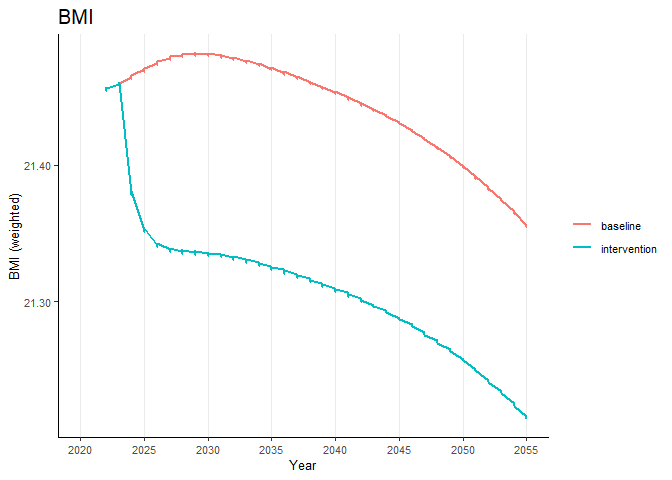
To plot the difference in the risk factor (say, “bmi”) for the weighted data, you can use the following code:
# Plot of difference in the risk factor "bmi"
riskfactors_diff("bmi",
                 data_weighted_rf_wide_collapse,
                 scale_y_continuous_limits = c(-0.148, 0),
                 scale_y_continuous_breaks = c(-0.148, -0.074, 0),
                 scale_y_continuous_labels = c(-0.148, -0.074, 0))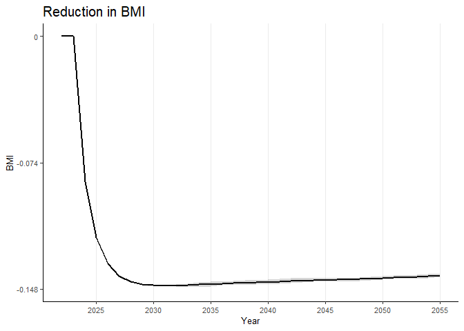
To plot the incidence difference for, say, “stroke”, you can use the following code:
data_weighted_ds_wide_diff <- gen_data_weighted_ds_diff(data_weighted,
                                                        configname = "default")
#> [1] "Loading the config file..."
#> [1] "Processing the data..."
#> [1] "Data processing complete."
inc_diff("stroke", data_weighted_ds_wide_diff)
#> Warning: Removed 170 rows containing missing values or values outside the scale range
#> (`geom_line()`).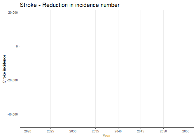
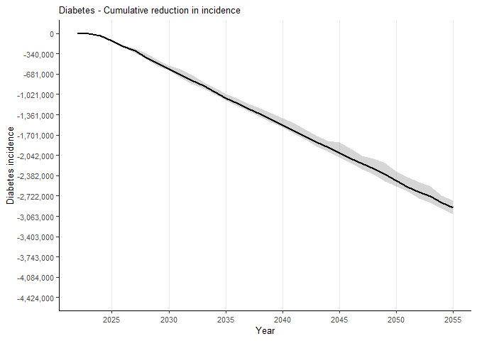
To plot the cumulative incidence difference for, say, “diabetes”, you can use the following code:
data_weighted_ds_wide_collapse <- gen_data_weighted_ds_cumdiff(data_weighted,
                                                               configname = "default")
#> [1] "Loading the config file..."
#> [1] "Processing the data..."
#> [1] "Data processing complete."
inc_cum("diabetes",
    data_weighted_ds_wide_collapse,
    scale_y_continuous_limits = c(-4424000, 0),
    scale_y_continuous_breaks = c(-4424000, -4084000, -3743000, -3403000, -3063000, -2722000, -2382000, -2042000, -1701000, -1361000, -1021000, -681000, -340000, 0),
    scale_y_continuous_labels = scales::comma(c(-4424000, -4084000, -3743000, -3403000, -3063000, -2722000, -2382000, -2042000, -1701000, -1361000, -1021000, -681000, -340000, 0))
  )
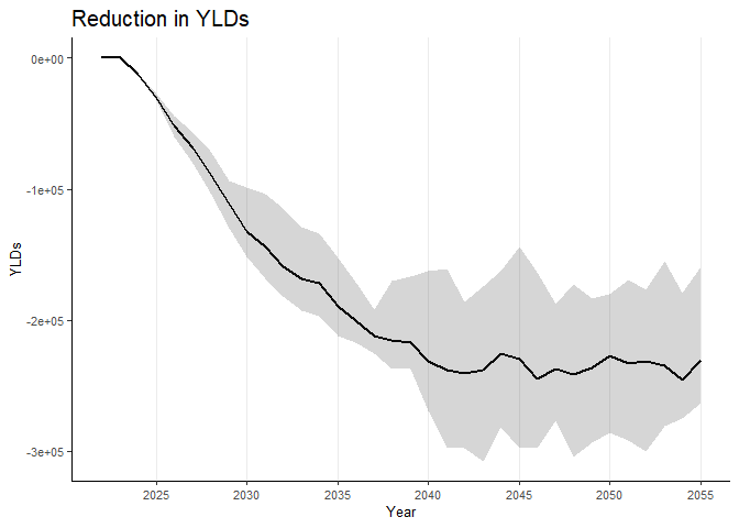
To plot burden of disease for, say, “yld”, you can use the following code:
data_weighted_bd_wide_collapse <- gen_data_weighted_burden(data_weighted,
                                                           configname = "default")
#> [1] "Loading the config file..."
#> [1] "Processing the data..."
#> [1] "Data processing complete."
burden_disease("yld", data_weighted_bd_wide_collapse)